TensorFlow Android App Debugging (1) -- Check Intermediate Results

To implement deep learning in smart phone, one can refer to the examples of TensorFlow Android app here. These examples include classifier, detector, voice recognition etc. Based on these frameworks, one can develop his own app with customized deep learning model. But during the process of development, on-target debugging is often needed to ensure that Android implementation generates identical results as offline processing. In this blog, we will provide a few tips for this debugging process.

One important step of debugging is that we need to know what happens in the device. For this purpose, Android provides logging function. Taking the file of TensorFlowImageClassifier.java as an example, it read in image data as:

    for (int i = 0; i < intValues.length; ++i) {
      final int val = intValues[i];
      floatValues[i * 3 + 0] = (((val >> 16) & 0xFF) - imageMean) / imageStd;
      floatValues[i * 3 + 1] = (((val >> 8) & 0xFF) - imageMean) / imageStd;
      floatValues[i * 3 + 2] = ((val & 0xFF) - imageMean) / imageStd;

To know their values, we can add log function as:

Log.i(TAG, "floatValues " + floatValues[i * 3 + 0] + " , " + floatValues[i * 3 + 1]+ " , " + floatValues[i * 3 + 2]);

Then by the device with PC by USB cable, each time we open the app, logcat will show these log information. This logging process can be extended to whatever variables we are interested in. Android Studio provides a logcat window. Another way for collecting log is to use adb instruction from command window. In my PC, it is
C:\Users\Nan\AppData\Local\Android\Sdk\platform-tools>adb logcat > logcat.txt


To implement deep learning neural network, TensorFlowImageClassifier.java loads a Tensorflow model used for image classification. To test our own model, we can exchange the default TensorFlow model to our own model. But sometimes the model may not work as expected. To debug this, not only the final output of the model is needed, sometimes we also want to dump out the intermediate results. The way to dump out intermediate results is to use fetch() function in TensorFlowInferenceInterface class. In the instruction below, batch_normalization_1/FusedBatchNorm_1 is a intermediate point in our customized TensorFlow model. fetch() function sends output of this intermediate point to the variable of outputs_intermediate. This variable has been initialized in earlier part of the code. To identify the labels of intermediate points of TensorFlow model such as batch_normalization_1/FusedBatchNorm_1, the tool of TensorBoard can be used.

inferenceInterface.fetch("batch_normalization_1/FusedBatchNorm_1", outputs_intermediate);

To support this Android debug process, there is often an offline processing flow which does things in parallel. This offline processing flow serves as reference for Android debugging. Below is snippet of Python code used for Tensorflow-based offline processing. Note that g_in is a variable for kernel weights and it is converted to kernel_conv2d_1, which is a numpy array. As a good first step for debugging, constant inputs can be injected for comparing outputs between Android and offline processing. Then we can inject the same image.

from tensorflow.python.platform import gfile
with tf.Session() as sess:
    # load model from pb file
    with gfile.FastGFile(wkdir+'/'+pb_filename,'rb') as f:
        graph_def = tf.GraphDef()
        graph_def.ParseFromString(f.read())
        sess.graph.as_default()
        g_in = tf.import_graph_def(graph_def, return_elements=['conv2d_1/kernel/read:0'])
    # write to tensorboard (check tensorboard for each op names)
    writer = tf.summary.FileWriter(wkdir+'/log/')
    writer.add_graph(sess.graph)
    writer.flush()
    writer.close()

    # inference by the model (op name must comes with :0 to specify the index of its output)
    tensor_output = sess.graph.get_tensor_by_name('import/dense_2/Softmax:0')
    tensor_input = sess.graph.get_tensor_by_name('import/input_1:0')
    tensor_intermediate = sess.graph.get_tensor_by_name('import/batch_normalization_1/FusedBatchNorm_1:0')

    kernel_conv2d_1=g_in[0].eval(session=sess)

    predictions = sess.run(tensor_output, {tensor_input: image_test})
    predictions_0 = sess.run(tensor_intermediate, {tensor_input: image_test})

Signal Processing Magic (4) -- DFT Analysis For A Tone

Tone is the most basic signal, yet it is quite useful. Because of its simplicity, tone is often used to calibrate a system. Thus it is important to know how to analyze a tone. In signal processing, spectrum analysis is an important tool, and spectrum is usually obtained through DFT.

For a tone with duration T, in time domain it looks like the plot below. As digitized signal, it has many samples; as complex waveform, it has both real and imaginary parts (blue curve for real part and red curve for imaginary part). Assuming sampling period Ts and in total N samples, T=N*Ts. Assuming Ts=1us and N=10000, T=10ms.

In the spectrum of a tone, there are a few important features to note. The first feature is that the delta between the amplitude of the main lobe and the amplitude of the side lobe next to the main lobe is 13.3dB. The second feature is that the width of the main lobe is 2/T. In this case, 2/T=200Hz. These features can be used for tone evaluation. For example, if the amplitude delta between the main lobe and the side lobe is larger than 13.3dB, this often means the tone is corrupted by a windowing function which can increases the amplitude delta.

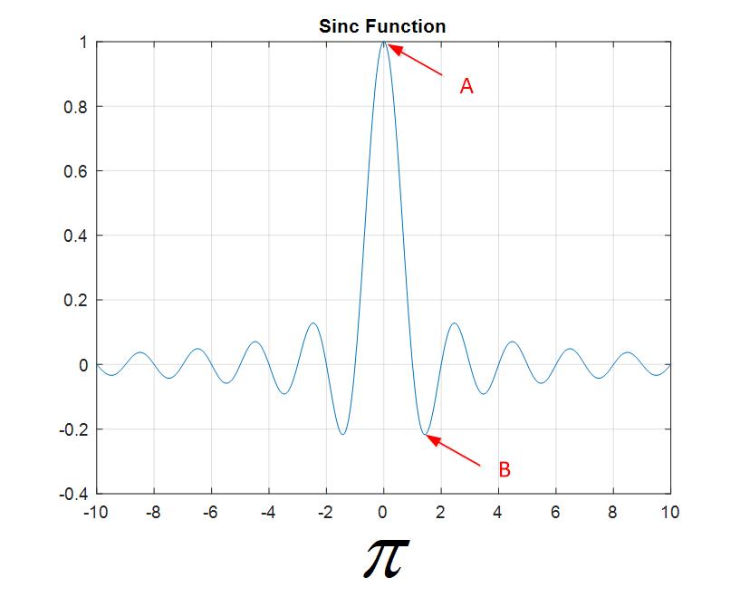
Both features can be explained by the relationship between rectangle waveform and sinc function. A tone with limited duration can be seen as imposing a rectangular window on a tone signal with infinite duration. If the tone signal has infinite duration, in spectrum it will show as an impulse. For a tone with limited duration, instead we will see a spectrum like above and this is due to frequency transform of a rectangular window in time domain. From signal processing 101, we know that a rectangular window in time domain can be transformed into a sinc function in frequency domain. sinc(x) = sin(x)/x. sinc(0) = 1 and it corresponds to the max amplitude of the main lobe (point A in the plot below). Point B corresponds to the max amplitude of the first side lobe in the spectrum. At point B, derivative of sinc(x) is 0. By numerical method, x point B can be found as 4.4934 (note that the x-axis of sinc function plot is scaled by Pi). And thus we find that the amplitude delta between point A and point B is exactly 13.3dB.

A PyTorch implementation of Image Segmentation Using UNet, Stratification and K-Fold Learning

This PyTorch script is the by-product of attending a Kaggle competition for image segmentation (https://www.kaggle.com/c/tgs-salt-identification-challenge). In this competition, the original images come from geological survey. The whole area of the original image can be divided into subarea with salt under the surface and subarea without salt under the surface (see original mask image). The competition goal is to segment test images into binary masks in which white means salt area and black means non-salt area.


Usually I wrote deep learning scripts using Keras. However, in this case, we choose to use PyTorch for pragmatic considerations. It is well-known that UNet [1] provides good performance for segmentation task. Part of the UNet is based on well-known neural network models such as VGG or Resnet. Compared with Keras, PyTorch seems to provide more options of pre-trained models. For instance, pre-trained model for Resnet34 is available in PyTorch but not in Keras. In order to capture the benefit of transfer learning, PyTorch is chosen over Keras for implementation.

For performance enhancement, when dividing training data to training set and validation set, stratification is used to ensure that images with various salt coverage percentage are all well-represented. In codes below, all training images are divided into 10 categories based on the percentage of their salt coverage ratio from low to high.

# Stratification: data binning based on salt size in mask. Divide each category to training and validation data
ind = np.arange(len(Y_train_shaped))
np.random.shuffle(ind)
coverage = []
for i in range(0, len(Y_train_shaped)):
  coverage.append(np.sum(Y_train_shaped[ind[i]]))

hist, bin_edges = np.histogram(coverage)
# In np.digitize, each index i returned is such that bins[i-1] <= x < bins[i]
# Need to increase the last bin_edges by 1 to avoid genarating a new category with digitize
bin_edges[len(bin_edges)-1] = bin_edges[len(bin_edges)-1] + 1
cindex = np.digitize(coverage,bin_edges)

In the next step, when training images are divided into training and validation set with 8:2 ratio, they are divided into 8:2 in each of these 10 salt-percentage-based categories. This is call stratification. In addition, we use 5-fold cross validation. It means the all training images are equally divided to 5 sets: 0/1/2/3/4. Then model 0 is trained with set 0 as validation and set 1/2/3/4 as training; model 1 is trained with set 1 as validation and set 0/2/3/4 as training; and so on. When all finished, we will have 5 trained models, and the final test results can be ensemble of the outputs of these 5 models. The benefit of K-fold learning is that all data is fully utilized and improved performance by ensemble; the drawback is higher computational complexity.

val_size = 2/10
for ii in range(5): #5-fold learning
    k = ii
    print('Training for '+str(k)+' of 5 fold starts!')
    train_idxs = []
    val_idxs = []
    for i in range(0,10):
      index_temp = ind[cindex==i+1]
      list_temp = index_temp.T.tolist()
      val_samples = round(len(index_temp)*val_size)
      if (k == 0):
          val_idxs = val_idxs + list_temp[:val_samples]
          train_idxs = train_idxs + list_temp[val_samples:]
      elif (k == 4):
          val_idxs = val_idxs + list_temp[4*val_samples:]
          train_idxs = train_idxs + list_temp[:4*val_samples]
      else:
          val_idxs = val_idxs + list_temp[k*val_samples:(k+1)*val_samples]
          train_idxs = train_idxs + list_temp[:k*val_samples] + list_temp[(k+1)*val_samples:]

In this implementation, we use AlbuNet [2], which is an variation of UNet.

    model = AlbuNet(pretrained=True, is_deconv=True);
    model.cuda();

    criterion = nn.BCEWithLogitsLoss()
    learning_rate = 1e-3
    optimizer = torch.optim.Adam(model.parameters(), lr=learning_rate)

AlbuNet is UNet based on Resnet34. Its topology is shown below:

To capture the whole implementation, source code of this implementation can be found here. You can run the script after downloading the dataset from Kaggle.


[1] Olaf Ronneberger et al, U-Net: Convolutional Networks for Biomedical Image Segmentation
[2] Vladimir Iglovikov and Alexey Shvets, TernausNet: U-Net with VGG11 Encoder Pre-Trained on ImageNet for Image Segmentation

Weight Distribution of MobileNet V1

Deep learning is increasingly used in devices with limited computing resource or limited power. For example, when deep learning is used in smartphone, power consumption becomes a primary concern. In order to reduce power consumption and increase computation efficiency, it is preferred to convert deep learning algorithm from floating point to fixed point. In order to convert an implementation from floating point to fixed point, first we need to know the distribution of parameters of the algorithm. In this blog, we choose a popular deep learning algorithm, MobileNet V1 [1], and plot the distributions of its weights.

As the first step, let us check the architecture of MobileNet V1 network:

import numpy as np
import matplotlib.pyplot as plt
import keras

base_model = keras.applications.mobilenet.MobileNet(weights='imagenet');

base_model.summary()

What this Python code does is to load the model of MobileNet V1 with the weights trained using ImageNet. base_model.summary() lists the summary of the network. The whole summary is long and we won't post it here. But the first a few lines look like this:

_________________________________________________________________
Layer (type)                 Output Shape              Param #
================================================
input_1 (InputLayer)         (None, 224, 224, 3)       0
_________________________________________________________________
conv1_pad (ZeroPadding2D)    (None, 225, 225, 3)       0
_________________________________________________________________
conv1 (Conv2D)               (None, 112, 112, 32)      864
_________________________________________________________________
conv1_bn (BatchNormalization (None, 112, 112, 32)      128
_________________________________________________________________
conv1_relu (ReLU)            (None, 112, 112, 32)      0
_________________________________________________________________
conv_dw_1 (DepthwiseConv2D)  (None, 112, 112, 32)      288
_________________________________________________________________
conv_dw_1_bn (BatchNormaliza (None, 112, 112, 32)      128
_________________________________________________________________
conv_dw_1_relu (ReLU)        (None, 112, 112, 32)      0
_________________________________________________________________
conv_pw_1 (Conv2D)           (None, 112, 112, 64)      2048
_________________________________________________________________
conv_pw_1_bn (BatchNormaliza (None, 112, 112, 64)      256
_________________________________________________________________
conv_pw_1_relu (ReLU)        (None, 112, 112, 64)      0
_________________________________________________________________


Each line of the summary includes three parts: the name of the layer, output shape of this layer, the number of parameters. Taking the example of the conv1 layer. "conv1 (Conv2D)" tells that its name is conv1 and it is doing 2D convolution. The output shape is "(None, 112, 112, 32) ", which means the output has 32 channels with image size 112x112 in each channel. The number of parameter is 864. 864 is calculated by 3x3x3x32=864 whereas 3x3 is the kernel size, 3 is the number of input channels, and 32 is the number of output channels. The next line of conv1_bn is for batch normalization. Batch normalization is proposed in [2] for faster convergence of neural network training. The equation of batch normalization is as below

\(y=\gamma\frac{x-E(x)}{\sqrt{Var(x)+\epsilon}}+\beta\)

Therefore, there are 4 parameters for each channel of batch normalization: \(\gamma\), \(\beta\), \(E(x)\), \(Var(x)\) (\(\epsilon\) is a constant, not a parameter). Since conv1_bn has 32 channels, it has 128 parameters.

MobileNet V1 is famous for decomposing a normal 2D convolution to a deep-wise convolution plus a 2D convolution with 1x1 kernel for reduced complexity. The layers of conv_dw_1 and conv_pw_1 in the summary show that. The layer of conv_dw_1 applied one and only one 3x3 kernel for convolution operation of each input channel. The resulted output shape is the same as the input shape. Since conv_dw_1 has 32 channels, the number of parameters is 32x3x3=288. Next, the conv_pw_1 layer is a 2D convolution with 1x1 kernel. Thus it has 1x1x32(input channels)x64(output channels)=2048. If a conventional 3x3 convolution is used for the same input and output, the number of parameters is 3x3x32x64 and it is much larger than 3x3x32+1x1x32x64. 

After going through the summary of the network, now it is time to plot its weights. To get the weights, we can use

W = base_model.get_weights();

The output W is a list with multiple elements. Each element is a numpy array. We can further print out the shape of each element.

for i in range(len(W)):
  print(W[i].shape)

Again, the printed outputs are long but it is sufficient to list the first dozen of lines to show how it work.
(3, 3, 3, 32)
(32,)
(32,)
(32,)
(32,)
(3, 3, 32, 1)
(32,)
(32,)
(32,)
(32,)
(1, 1, 32, 64)
(64,)
(64,)
(64,)
(64,)

The first line is for the weights of conv1 layer with 3x3x3x32 parameters. The next four lines are for the conv1_bn layer. After checking the source code for how weights are added to the model, we are convinced that the four lines are in turn for \(\gamma\), \(\beta\), \(E(x)\) and \(Var(x)\). The remaining lines of the printout can be mapped to the network layers too.

When plotting the distribution of weight, we plot it layer by layer. For instance, we can plot the distribution of conv1_bn layer weights by using:

plt.hist(W[0].flatten())

Figure below shows the distribution of convolution layers of MobileNet V1 model trained with ImageNet data:

Distributions of  convolution weights

The plot of weight distribution shows that the weight distribution are mostly symmetric. The dynamic range changes from [-0.5,0.5] in conv_pw_13 to [-30, 25]  in conv_dw_1.

Next we plot the distribution of weights used in batch normalization layers. The formula of batch normalization can be simplified to

\(y=\gamma\frac{x}{\sqrt{Var(x)+\epsilon}}+\beta-\gamma\frac{E(x)}{\sqrt{Var(x)+\epsilon}}\)

We call \(\frac{\gamma}{\sqrt{Var(x)+\epsilon}}\) scale and call \(\beta-\gamma\frac{E(x)}{\sqrt{Var(x)+\epsilon}}\) bias.

Distribution of batch normalization scales

Distribution of batch normalization bias

It is observed that the scales of batch normalization are mostly positive. The dynamic range of bias distribution changes from [-2.5, 2.5] to [-30, 25], which seems to be less than the dynamic range of weight distribution of convolution layers.

Source code for this analysis can be found here.



[1] Andrew G. Howard et al, MobileNets: Efficient Convolutional Neural Networks for Mobile
Vision Applications
[2] S. Ioffe and C. Szegedy, Batch Normalization: Accelerating Deep Network Training by Reducing Internal Covariate Shift

Is Python Image resize() Function Reversible?

During image processing tasks, frequently we need to change the image size. For instance, the original image size is 100x100 but certain neural network needs input size of at least 255x255. That requires us to interpolate, which increases the image size. On the other hand, we might get some high-definition images with size much larger than 255x255. For these images, we will perform image decimation to reduce the image size. For both image interpolation and decimation, we can use resize() function defined in skimage.transform Python module.

Some tasks require first changing image size from 100x100 to 255x255, processing it, and then changing it back to 100x100. These kinds of tasks motivate the study of this article. The question we ask is this: if we change an image of size x0-by-y0 to size x1-by-y1 and then change it back to the original size, will the newly generated image the same as the original image? If they are the same, we call the resize() function to be reversible; if not, we call it not reversible. If it is reversible, that means the whole image conversion process does not add any additional noise, which in general is a good thing to have.

First let us see what is offered in skimage resize() function. Note that the manual use the word "interpolation" for all image size change no matter it becomes larger or smaller. According to the manual, six interpolation methods are provided in the function controlled by a parameter named "order". According to the manual:

The order of interpolation. The order has to be in the range 0-5:

• 0: Nearest-neighbor
• 1: Bi-linear (default)
• 2: Bi-quadratic
• 3: Bi-cubic
• 4: Bi-quartic
• 5: Bi-quintic

Among these methods, nearest-neighbor, bi-linear and bi-cubic methods are probably the most well-known approaches with increased complexity. For each pixel in the new image, nearest-neighbor method identifies the pixel in the old image the closest to the new pixel and then make the new pixel identical to the old pixel. Nearest-neighbor method only needs one pixel in the old image for interpolation. By comparison, bi-linear method needs four pixels in the old image. Bi-linear interpolation can be explained by the figure below borrowed from wiki. To generate the new pixel P, bi-linear interpolation uses four points in the original image (Q11, Q12, Q21, Q22). Linear interpolation is performed first in x dimension and then y dimension.


Bi-cubic interpolation is more complicated. Bi-cubic represents interpolation using a polynomial with 16 coefficients. To figure out these coefficients, it needs 16 points from the original image as inputs. The bi-cubic equation is as below:
\[f(x,y)=\begin{bmatrix} x^{3}&x^{2}&x&1\\  \end{bmatrix}\begin{bmatrix} a_{3,3}&a_{3,2}&a_{3,1}&a_{3,0}\\ a_{2,3}&a_{2,2}&a_{2,1}&a_{2,0}\\a_{1,3}&a_{1,2}&a_{1,1}&a_{1,0}\\ a_{0,3}&a_{0,2}&a_{0,1}&a_{0,0}\\ \end{bmatrix}\begin{bmatrix} y^{3}\\ y^{2}\\y\\1 \end{bmatrix}\]

In our experiments, we will take two pictures, one for image and another for mask. Image and mask are common settings for image segmentation task. These two original pictures are both of size 101x101. Then we will resize these two to 128x128 and then convert them back to the orignal size of 101x101. The evaluation metric is sum(abs(original image - output image from two resize operations)). When this summation equals to zero, we call the image resize operation reversible. We will evaluate three interpolation approaches: nearest distance, bi-linear, bi-cubic.

Original: left side is the original image while the right side is mask. Mask is binary. Each pixel of mask is either 0 or 1.

Nearest-neighbor: What is shown here is the delta between original and the output of two resize operations using nearest-neighbor interpolation. For nearest-neighbor method, delta is zero for both image and mask. The reason for zero delta is this: nearest-neighbor method is bi-directional. When a new pixel is nearest neighbor to an old pixel, when resize back, the old pixel is the nearest neighbor to the new pixel as well. That means resize operation using nearest-neighbor method is reversible.

Bi-linear: bi-linear interpolation is not reversible. As the diagram below shows, the delta between original and resize output is not all zero. Since mask is binary, the delta for mask in the right is more significant than the image in the left. For the picture in the left, non-zero points show at image boundary and also scatter sporadically over the whole image. For the picture in the right, non-zero points shows in the boundary and also along the border between all-zeros area and all-ones area of the original mask image.

Bi-cubic: bi-cubic has the same issue as bi-linear. However, based on metric of the sum of square error, bi-cubic generates less delta than that of bi-linear. In term of image in the left, the sum square error is 3.14 for bi-linear versus 0.32 for bi-cubic; in term of mask in the right, the sum square error is 13.14 for bi-linear versus 4.78 for bi-cubic.

What this study tells us is that from the perspective of reducing additional noise caused by resize forward and backward, the best choice is nearest-neighbor interpolation since it does not introduce any additional noise. Other than that, bi-cubic is also a good choice although the computation complexity is higher. Note that when applying resize() function, bi-linear is the default. Sample script used in this study can be found here.

My $1000 Deep Learning Box

For machine learning enthusiastic, it is always good to have their own box to do deep learning number crunching. The easiest way is probably to purchase a desktop from Dell, HP or other vendors, and then add a GPU on top. I have considered this option but eventually gave it up. One reason for abandoning this idea is that it is hard to customize a commercially available desktop. For instance, if you want a 750W power supply to ensure GPU won't be short of power or need a motherboard which can support two GPUs, it is not easy to find such a desktop in the market with acceptable price. There are other reasons as well. I want to use a Linux computer dedicated for machine learning purpose but most of the computers available in the market come with Window OS. Therefore, after some contemplating, I decide to assemble my own computer, for which I have not done before.

Hardware

After searching in Internet, I found lots of useful information. In particular, I took good reference from the computer component list provided in this blog. But I also made some modifications on top of Yanda's list. Here is the list of components I am using:

1. EVGA GeForce GTX 1060 SC GAMING, ACX 2.0 (Single Fan), 6GB GDDR5, DX12 OSD Support (PXOC), 06G-P4-6163-KR   (A GPU not as fancy as GTX1080. But it is a fair choice for personal usage and can be upgraded later. $278)

2. ASUS ROG Strix Z370-G Gaming LGA1151 (Intel 8th Gen) DDR4 DP HDMI M.2 Z370 Micro ATX Motherboard with onboard 802.11ac WiFi, Gigabit LAN and USB 3.1 (Motherboard recommended by Yanda. This board can support up to 2 GPUs, which means there is room to expand. $189)

3. WD Blue 3D NAND 500GB PC SSD - SATA III 6 Gb/s M.2 2280 Solid State Drive - WDS500G2B0B (this 500GB SDD drive is also recommended by Yanda. I like it since this SDD drive can be embedded into the Z370-G motherboard. $95)

4. Corsair Vengeance LPX 16GB (2x8GB) DDR4 DRAM 3200MHz C16 Desktop Memory Kit - Black (CMK16GX4M2B3200C16) (16GM DRAM, 170$)

5. Intel 8th Gen Core i5-8400 Processor (For budget purpose, I did not purchase i7 but instead settled with an 8th gen i5 processor, $180)

6. EVGA Supernova 750 G3, 80 Plus Gold 750W, Fully Modular, Eco Mode with New HDB Fan, 10 Year Warranty, Includes Power ON Self Tester, Compact 150mm Size, Power Supply 220-G3-0750-X1 (this 750W power supply is recommended by Amazon. It seems to be a quite popular choice and is so far so good for me. $97)

7. Thermaltake Versa H15 SPCC Micro ATX Mini Tower Computer Chassis CA-1D4-00S1NN-00 (This case is also recommended by Amazon. I think any case with good reviews and supports microATX standard should do the job. $41)

All seven components add to $1050. If one chooses better CPU (like i7), better GPU (like GTX1080), or more than one GPU, the budget for this box will increase. But it also shows the benefit of DIY since it is fairly easy to tune the computer setting according to your own budget and needs.

I assembled everything myself. Even though it is the first time I did that, the whole process seems not to be that difficult. And my computer already starts running and it seems that I have not blew up anything. However, you want to read the manual especially the motherboard manual carefully before starting. Youtube education videos can also be quite benefitial.

Software

I installed Ubuntu Linux in my computer. Ubuntu website provides a good tutorial of how to create bootable USB stick for Ubuntu. I follow up that direction to install a Ubuntu 18.04 and everything works fine. During my installation process, I did not allow installing 3rd software out of the concern that it can mess up with Nvidia GPU installation done later.

The trickiest thing during the whole procedure of box assembly is installing CUDA. CUDA support for Linux is far from perfect. As of the time I wrote this blog, CUDA website only support Ubuntu 17 and 16, but not Ubuntu 18. Internet search returns lots of results of how to install CUDA in Ubuntu yet many of them are confusing especially for a Ubuntu newbie like me. For example, I had followed some recommendation to turn off X-server and it ends up with endless black screen. What eventually saves me is this blog.  The author lays out a relatively straightforward path to install CUDA in Ubuntu 18.04 and most importantly, it works! The only thing missing in that blog is how to install Nvidia driver version 390. For Nvidia driver installation, this discussion tells how to do it. It shows two ways and below is what I did. After driver installation done, remember to use nvidia-smi to verify the installation.

$ sudo add-apt-repository ppa:graphics-drivers/ppa
$ sudo apt update

$ sudo apt install nvidia-390

After installing CUDA, CUDNN, Tensorflow, you are still a few steps away from running your first deep learning code in the box. For example, you may want to install keras and other Python packages. However, these steps are straightforward. Finally, you should observe a keras or tensorflow sample code running on GPU and it calls a good end to your day.

Image Augmentation For Deep Learning Without Using ImageDataGenerator

Image augmentation is an important technique used in image-related deep learning to reduce overfitting. Neural networks used in deep learning often have millions of parameters and they are good at memorizing training data. That means the converged network model is good at training data but bad at other data such as validation or test data. We call this phenomenon "overfitting" since the model fits too well to the training data. There are multiple ways to alleviate overfitting issue. One of them is image augmentation. Image augmentation means that instead of feeding training data only, we also feed randomly tilted, shifted, flipped or scaled training images to the model. Randomized images make it harder for the neural network to memorize the training data. Therefore, it may reduce the gap between training accuracy and validation accuracy. Ultimately, data augmentation technique could improve the validation accuracy.

Some deep learning library like Keras provides good built-in function for image augmentation called ImageDataGenerator. This tool is fairly easy to use and fits well with Keras framework. However, if other deep learning library like PyTorch is used, ImageDataGenerator is not available and users need to develop its own image augmentation code. In this article, we will demonstrate how to do that. In particular, we will show an example of how to augment images for the task of image segmentation and this task involves a pair of images: image and mask. Similar method can also be used to augment single image.

The baseline of augmentation code comes from EKami's work related to Kaggle carvana challenge (https://github.com/EKami/carvana-challenge/blob/original_unet/src/img/augmentation.py). This code is an excellent example of how image augmentation should be done. On top of it, we made the following improvements:
1. The original function of augment_img(img, mask) seems not to always change image and mask at the same time. Digging deeper, random_shift_scale_rotate() function are called twice, one for image and another for mask. However, np.random.random() used in that function can have different values for image and for mask. That seems to explain why image and mask are not always modified simultaneously. To address this issue, we create a new function named augment_img_reshape(). In this new function, a common random number is always shared between image and mask conversion. That guarantees that both images are modified simultaneously.
2. To favor deep learning, the input image are often modified to channel-first format as (im_chan, im_width, im_height) for image and (1, im_width, im_height) for mask. This format does not match with the format required by the baseline code. Instead, we add format conversion support to augment_img_reshape().

To show an example, running image_augmentation.py stored in here generated both original image/mask and image/mask after augmentation. One example is shown below. Note that since it is a random event, sometime the images before and after augmentation are identical.