Wednesday, May 25, 2016

ICP Algorithm for Point Cloud Stitching

ICP stands for Iterative Closest Point algorithm. It is a well-known algorithm used to align two point clouds.

Iterative Closest Point


  1. Search for correspondences.
  2. Reject bad correspondences.
  3. Estimate a transformation using the good correspondences.
  4. Iterate.

Many tutorials are available online for ICP algorithm such as http://www.cs.technion.ac.il/~cs236329/tutorials/ICP.pdf

The popular PCL library for point cloud processing provides ICP class here: http://pointclouds.org/documentation/tutorials/iterative_closest_point.php

Here is another example of Matlab implementation for ICP: http://www.csse.uwa.edu.au/~ajmal/code/icp.m

Despite the popularity of ICP, when using it, I find that the result is not always satisfactory. The biggest problem is that there is no guarantee that ICP will converge to global optimum. In practice, it often converges to local optimum. As shown in the picture below, when point clouds A and B merge, depending on the starting positions, it is possible that ICP only merges part of the clouds.


Tuesday, May 24, 2016

Use Rodrigues' Rotation to Convert 3D data to 2D

In this blog, we introduce how Rodtrigues' rotation formula can be use to convert 3D data to 2D. Let us assume that we have a bunch of 3D points, and we want to project them to x/y axis plane for easier analysis. The Matlab code below implements this function.

clear all; close all;

% collect 3D points 
xyz = [-0.485 0.130 1.489
    0.008 0.134 1.464
    -0.008 0.425 1.458
    -0.465 0.414 1.470
    -0.489 0.136 1.483
    -0.465 0.412 1.470
    0.006 0.137 1.464];

% Model them as a plane in 3D using least square method
[h,l]=size(xyz);
coef = inv(xyz'*xyz)*(xyz'*ones(h,1));
coef_unit = (coef/sqrt(coef'*coef)).';

% Rodrigues' rotation formula
in0 = coef_unit;
in1 = [0 0 1];
% Reference
in0Norm = in0 ./ sqrt(in0*in0.');
in1Norm = in1 ./ sqrt(in1*in1.');
axisRaw = cross(in0Norm, in1Norm);
axis = axisRaw./sqrt(axisRaw*axisRaw.');
angle = acos(dot(in0Norm, in1Norm));
M = [axis(1)^2+(1-axis(1)^2)*cos(angle) axis(1)*axis(2)*(1-cos(angle))-axis(3)*sin(angle) axis(1)*axis(3)*(1-cos(angle))+axis(2)*sin(angle);
axis(1)*axis(2)*(1-cos(angle))+axis(3)*sin(angle) axis(2)^2+(1-axis(2)^2)*cos(angle) axis(2)*axis(3)*(1-cos(angle))-axis(1)*sin(angle);
axis(1)*axis(3)*(1-cos(angle))-axis(2)*sin(angle) axis(2)*axis(3)*(1-cos(angle))+axis(1)*sin(angle) axis(3)^2+(1-axis(3)^2)*cos(angle)];
    
% Project 3D points to 2D plane with z=0 
xyz_ortho = xyz - xyz*coef_unit.'*coef_unit;   
xyz_prj = M*xyz_ortho.';

Let us walk through the code step-by-step.

Step 1: A plane in 3D space can be characterized as \( a x + b y + c z = 1 \). Assuming that matrix \(X\) has all 3D points: \[ X = \begin{bmatrix}
    x_{0}       & y_{0} & z_{0}  \\
    x_{1}       & y_{1} & z_{1} \\
    ...              & ...        &...\\
    x_{N}       & y_{N} & z_{N}
\end{bmatrix}\]
Then least square estimator for [a b c] is \( coef = (X'X)^{-1}(X'h)\) where \(h = [1 1 ... 1]'\) and \(X'\) is the transpose of \(X\). Normalized version of coef is called coef_unit.

Step 2: Use Rodrigues' rotation formula to find the matrix \(M\) which can rotate coef_unit to [0 0 1].

Step 3: First we project all 3D points to a plane characterized by [x y z]*coef_unit = 0. This is achieved by:
xyz_ortho = xyz - xyz*coef_unit.'*coef_unit;   
The last step is to use rotation matrix \(M\) to reduce the dimension of xyz_ortho to 2D. After the rotation, all z-axis elements in xyz_prj are 0's.


Monday, May 23, 2016

Vector Kalman Filter

Kalman filter is one type of statistical filtering. It was invented in 1970's and has been widely used till now. There are different variations of Kalman. We focus on vector Kalman filter here.

For system model, we have two equations:
\[s[n]=\textbf{A}s[n-1]+\textbf{B}u[n] \qquad (1)\]
\[x[n]=\textbf{H}[n]s[n]+w[n] \qquad (2)\] 
\(s[n], x[n], u[n], w[n]\) are vectors; \(\textbf{A}, \textbf{B}, \textbf{H}[n]\) are matrices. \(s[n]\) is the signal and what we want to detect. Equation (1) shows that the signal in time n and time n-1 are correlated. \(s[n]\) is generated by \(s[n-1]\) plus a noise \(u[n]\). \(u[n]\) is white noise with \(N(0, \textbf{Q})\). But equation (1) alone does not give a good estimate of \(s[n]\). As time goes by, \(u[n]\) keeps adding noise to the estimate and eventually will render it unusable. That is where equation (2) comes into the picture. \(x[n]\) in equation (2) is observation. In each moment, the observation of \(x[n]\) is used to refine the estimate of \(s[n]\). \(x[n]\) is also corruptedby noise \(w[n]\), which has spectral density of \(N(0,\textbf{C}[n])\).

Now the problem comes: how should we utilize the observation? If we just have equation (2) but not equation (1), then MMSE or LS estimators are natural choices. But with equation (1), these estimators will be sub-optimal since they fail to consider the previous results of s. Kalman filter was invented to fully utilize the information given in both equations. Under Kalman filter, the estimate of s, s_hat, is derived from equation (1) but then corrected by the observation in equation (2).

The first step of Kalman filter is prediction:
\[\hat{s}[n|n-1]=\textbf{A}\hat{s}[n-1|n-1]\qquad(3)\]
The new MSE of \(\hat{s}[n|n-1]\) becomes
\[\textbf{M}[n|n-1]=\textbf{AM}[n-1|n-1]\textbf{A}'+\textbf{BQB}'\qquad(4)\]
where \(\textbf{A}\)' is the transpose of conjugate of the matrix \(\textbf{A}\). Equation (4) shows that without correction, MSE will keep growing due to \(\textbf{BQB}'\).

For correlation, we uses MMSE filter, which is the best known filter to reduce Mean Square Error. The formula for MMSE filter is
\[\textbf{K}[n]=E(x[n]s[n]')(E(x[n]x[n]')^{-1}\qquad(5)\]
where \((.)^{-1}\) means matrix inverse. Thus
\[\textbf{K}[n]=\textbf{M}[n|n-1]\textbf{H}[n]'(\textbf{H}[n]\textbf{M}[n|n-1]\textbf{H}[n]'+\textbf{C}[n])^{-1}\qquad(6)\]

Then the correction formula for Kalman becomes
\[\hat{s}[n|n]=\hat{s}[n|n-1]+\textbf{K}[n](x[n]-\textbf{H}[n]\hat{s}[n|n-1])\qquad(7)\]
\(x[n]\) is supposed to be a good estimation of \(\textbf{H}[n]\hat{s}[n|n-1]\). The difference between these two are used to correct \(\hat{s}\).
Correction should reduce MSE. The new MSE is
\[E\big((s[n]-\textbf{K}[n]x[n])(s[n]-\textbf{K}[n]x[n])'\big)\]
Based on the orthogonality rule of MMSE filter,
\[E((s[n]-\textbf{K}[n]x[n])x[n]')=0\]
Therefore, MSE can be modified to be

E((s[n]-K[n]x[n])(s[n]-K[n]x[n])')
=E((s[n]-K[n]x[n])s[n]')
=E(s[n]s[n]')-K[n]E(x[n]s[n]')
= (I-K[n]H[n])M[n|n-1]
=M[n|n]

I don't want to drive people to sleep but this is how things are. Kalman filtering is not easy. To use Kalman, you need to come out with the models of A, B, C, Q, H. Depending on the size of s and x, you may also need to inverse a large matrix. 

Steven Kay's classic book: Fundamentals of statistical signal processing -- estimation theory, has one chapter dedicated to Kalman filter. You can refer to that book for more knowledge of Kalman filtering.


Saturday, April 9, 2016

Deep Dive Into PulsedLight LIDAR-Lite V2 Device

LIDAR-Lite V2 Device is produced by http://pulsedlight3d.com/  This excellent device uses laser to measure the distance. The max distance is 40m. You can use it for both indoor and outdoor. And it is quite convenient to hook it up with open-source platform like Arduino. As the name suggested, its main usage is for LIDAR sensor. You can mount it to a robot or a drone to collect surrounding information. But people also use it for other purposes like generating point cloud.


This is what we see when open the device. Inside it has two parts: the upper part is the laser diode, which is the transmitter. The lower part is receiver, which can sense the laser light. It works like radar: the upper part sends a laser beam. The beam is reflected by object and the lower part detects the reflection. By correlating the signal sent and signal received, it can identify the peak of correlation and derive the distance based on the peak location. When the object moves farther, the reflection peak will be detected later. 


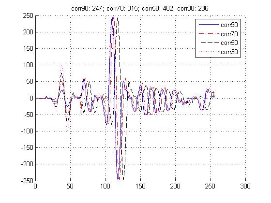
The SW library of LIDAR Lite allows to retrieve the correlation values. For each correlation, it has 256 elements. The plot below includes correlation of a few distance measurements. "corr50" curve has the max distance of 4.82m (482cm). Clearly the correlation peak occurs later for larger distance.

lidar_lite_corr.jpg

Monday, April 4, 2016

Quaternion-Based Rotation in OpenGL

This is yet another blog about quaternion. Assuming that we have quaternion [q0, q1, q2, q3]. Can we directly use it to rotation object in OpenGL? The answer is yes. At first, let us normalize this quaternion (written with Java)

     norm = (float) Math.sqrt(q0*q0 + q1*q1 + q2*q2 + q3*q3);
    if (norm == 0)
    {
    return 0;
    }
    else
    {
    q0 = q0 / norm;
    q1 = q1 / norm;
    q2 = q2 / norm;
    q3 = q3 / norm;
    }

Then, glRotatef function in OpenGL is a natural fit for rotation using quaternion.
 
        // Rotate the object according to quaternion
        theta = (float) (Math.acos(q0) * 2);
        
        aNorm = (float) Math.sqrt(q1 * q1 + q2 * q2 + q3 * q3);
        if (aNorm != 0)
        {
        gl.glRotatef(theta*180f/PI, q1/aNorm, q2/aNorm, q3/aNorm);
        }
        else
        {
        gl.glRotatef(theta*180f/PI, q1, q2, q3);
        }

Note that except for quaternion, glRotatef can also be used for rotation along x, y or z axis. In that way, glRotatef needs to be called three times instead of once with quaternion-based method.

    glRotatef(xRot , 1.0, 0.0, 0.0);
    glRotatef(yRot , 0.0, 1.0, 0.0);
    glRotatef(zRot , 0.0, 0.0, 1.0);

Sunday, April 3, 2016

How To Find A Point's Screen Correspondence in OpenGL

To project a point, we can use gluProject function. What the function does is to project a 3D coordinate to the window screen.

GLfloat x,y,z;
double wx,wy,wz,pixel_x,pixel_y;
double modelMatrix[16];
double projMatrix[16];
GLint viewport[4];

// To find the projection
glGetDoublev(GL_MODELVIEW_MATRIX,modelMatrix);
glGetDoublev(GL_PROJECTION_MATRIX,projMatrix);
glGetIntegerv(GL_VIEWPORT,viewport); 
gluProject(x, y, z, modelMatrix, projMatrix, viewport, &wx, &wy, &wz); 

If we want to compare the screen coordinate of the point with the location of the mouse, a little bit extra processing is needed before comparing with event->x()/y(), which are mouse locations.

pixel_x = wx;
pixel_y = viewport[1] + viewport[3] - wy;
dist = (pixel_x - event->x()) * (pixel_x - event->x()) + (pixel_y - event->y()) * (pixel_y - event->y());

How To Zoom In in OpenGL + Qt


Recently I am working on a project which utilizes Qt5.3+OpenGL. I need to implement a function in which by spinning the mouse wheel, the 3D object in OpenGL view can be enlarged or shrunk. After some research, it is found that we can implement the function in two ways: glScaled or  glOrthof.

Approach 1: glScaled

glScaled function scales the x, y, z by a factor. In my implementation, all three axis are scaled by the same factor.

First, the mouse wheel function is written in such a way that wheel rotation changes a zoom factor named zoomScale. After that, it will call the paintGL() function where galScaled is embedded.

void GLWidget::wheelEvent(QWheelEvent *event)
{
QPoint numDegrees = event->angleDelta();
if (numDegrees.y() < 0)  zoomScale = zoomScale/1.1;
if (numDegrees.y() > 0)  zoomScale = zoomScale*1.1;

updateGL(); // call paintGL()
}

In paintGL() function, galScaled() is called and zoomScale is used to scale x, y, and z axis. We should note that in order to avoid unnecessary clipping, the near and far planes of OpenGL view need to be set with some redundancy.

void GLWidget::paintGL()
{
    glClear(GL_COLOR_BUFFER_BIT | GL_DEPTH_BUFFER_BIT);
    glLoadIdentity();
    glScaled(zoomScale, zoomScale, zoomScale);
    glRotatef(xRot / 16.0, 1.0, 0.0, 0.0);
    glRotatef(yRot / 16.0, 0.0, 1.0, 0.0);
    glRotatef(zRot / 16.0, 0.0, 0.0, 1.0);


Approach 2: glOrthof

glOrthof function defines a box where the objects are shown in OpenGL. The box has left, right, up, down, near, far boundaries. Again, we starts from the wheelEvent function which calls resizeGL().

void GLWidget::wheelEvent(QWheelEvent *event)
{
QPoint numDegrees = event->angleDelta();
if (numDegrees.y() < 0)  zoomScale = zoomScale/1.1;
if (numDegrees.y() > 0)  zoomScale = zoomScale*1.1;
GLint viewport[4];
glGetIntegerv(GL_VIEWPORT,viewport); 
resizeGL(viewport[2], viewport[3]);

updateGL(); // call paintGL()
}

In resizeGL, zoomScale is used to adjust the boundaries in x and y directions. In this way, we can also implement the zoom in/out functions.

void GLWidget::resizeGL(int width, int height)
{
    int side = qMin(width, height);
int range = 1000;
    //glViewport((width - side) / 2, (height - side) / 2, side, side);
glViewport(0, 0, width, height);

    glMatrixMode(GL_PROJECTION);
    glLoadIdentity();

    glOrthof(-0.5*range*zoomScale, +0.5*range*zoomScale, -0.5*height/width*range*zoomScale, +0.5*height/width*range*zoomScale, -5*range, +5*range);

    glMatrixMode(GL_MODELVIEW);
}